Biological LLM Evo 2: Getting Started

Large language models have transformed knowledge work with a simple idea: Train a model to predict the next token using a lot of data. Similarly, the same idea is poised for a fundamental shift in biology which will open up new ways to do computational biology.

However, we will first need to resolve some challenges peculiar to biological sequence data. Take the human genome as an example. It has 6 billion base pairs arranged hierarchically. Two sequences millions or even billions of base pairs apart can interact physically and functionally.

Evo 2, a groundbreaking biological foundation model from the Arc Institute, is the latest model to take on this challenge. Built on a modified attention architecture with up to 40 billion parameters and a massive 1-million-token context window. By training on over 9 trillion nucleotides, Evo 2 has learned to predict the effects of genetic mutations with zero-shot accuracy and can even generate functional genomic sequences from scratch.

In this article, I will cover:

• Installing Evo 2
• Mutation prediction with zero-shot learning
• Mutation prediction with few-shot learning

Install Evo 2

Since Evo 2 is a deep learning model, you will save yourself a lot of trouble by installing it on a Linux environment with an Nvidia GPU card. If you have a Windows system, switch to WSL (Windows Subsystem for Linux) before installing Evo 2.

Install Conda

Download miniconda if you don’t have Conda already.

wget https://repo.anaconda.com/miniconda/Miniconda3-latest-Linux-x86_64.sh

Install Conda.

bash Miniconda3-latest-Linux-x86_64.sh

Proceed with initialization: Yes

conda config --set auto_activate_base false

Install Evo 2

Clone the Evo 2 repository.

git clone https://github.com/arcinstitute/evo2
cd evo2

Create a Conda environment with Python 3.12.

conda create -n evo2 python=3.12

Activate the conda environment.

conda activate evo2

Install the Transformer Engine and Flash Attention prerequisites.

conda install -c nvidia cuda-nvcc cuda-cudart-dev
conda install -c conda-forge transformer-engine-torch=2.3.0
conda install psutil
pip install flash-attn==2.8.0.post2 --no-build-isolation

pip install -e .

You need gcc to compile the code. Run the following command to check if you have it already.

which gcc

If not, install gcc with the following commands.

sudo apt-get update
sudo apt-get install build-essential

Verify the installation.

python -m evo2.test.test_evo2_generation --model_name evo2_7b

You should see the completion of the script with a PASS.

First Project: BRCA1 mutation prediction

A good first project is to use Evo 2 to predict the effect of a single nucleotide mutation on the BRCA1 gene (BReast CAncer gene 1). The gene encodes the protein that helps repair damaged DNA. A patient is more likely to have breast or ovarian cancers if she has a mutation in this gene that produces a defective copy of this protein.

All mutations of the BRCA1 gene are characterized by a genome editing study, which scored each mutation on how it impaired the DNA-repairing protein.

Probability of a sequence

Since Evo 2 have learned the natural pattern of DNA sequences, it can calculate how “normal” the mutated BRCA1 sequence is.

The calculation is demonstrated in the BRCA1 zero-shot learning notebook, which calculate the likelihood of the sequence after the mutation.

The Evo 2 is an autoregressive model like ChatGPT and Gemini. It predicts the probability of the next base. For example, what is the probability of seeing the sequence ‘TACG’ according to the Evo 2 model? That would be:

P(TACG) = P(T) P(A|T) P(C|TA) P(G|TAC)

This is what happen when you put the sequence TACG through the model.

1. The first token is <BOS> (Beginning of sequence). So P(T) is actually the probability of getting T after <BOS> (P(T|<BOS>)).
2. The model processes the first token <BOS> and output the probabilities of the next token. For example, T is 20%, A is 20%, C is 30%, and G is 30%. In this case, P(T) = 20%.
3. Now, we have two tokens <BOS>T to feed into the model. The model predicts the probabilities of the next token. E.g. T is 10%, A is 15%, C is 30%, and G is 35%. So, P(A|T) = 15%.
4. Feed <BOS>TA into the model. The model again predicts the probabilities of the next token. E.g. T is 20%, A is 15%, C is 25%, and G is 40%. So P(C|TA) = 25%.
5. Finally, feed <BOS>TAC into the model. The model predicts the probabilities of the next token. E.g. T is 40%, A is 25%, C is 15%, and G is 20%. So P(G|TAC) = 20%.

So we can calculate P(TACG) = P(T) P(A|T) P(C|TA) P(G|TAC) = 20% * 15% * 25% * 20% = 0.15%

Mutation score

This probability is high when the sequence looks like those in the training data. Lower when it looks unfamiliar.

If a mutation in the BRCA1 gene lowers the probability of a sequence, it looks less like something that would appear naturally. This implies a loss-of-function mutation because living organisms don’t usually carry them.

So, the notebook calculates the Evo 2 mutation (delta) score as P(mutated sequence) – P(original sequence). The lower the score is, the more likely the mutation disrupts the function of the DNA-repairing protein.

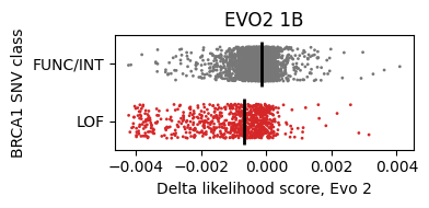
Predicting mutation classification

The experimental data measure the mutation’s disruptiveness and indicate whether it is benign or causes loss of function.

Running through the notebook gives a comparison between the model’s prediction (x-axis) vs the experimental classification (y-axis). Here, FUNC/INT indicates the mutation is benign and doesn’t affect the protein’s function. LOF stands for loss-of-function.

Benign mutations have higher delta scores on average, as expected, because we are more likely to see them in nature.

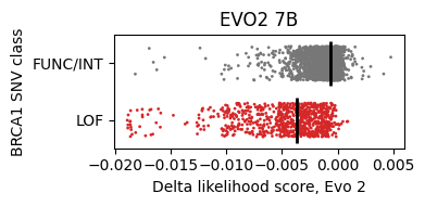
Modification 1: Using the bigger 7B model

The notebook uses the Evo 2 Base model with 1 billion parameters. Would repeating the numerical experiment with a bigger model produce a better result?

Changing this:

model = Evo2('evo2_1b_base')

To:

model = Evo2('evo2_7b')

And rerun the notebook. The two distributions seem to be more separable.

The area under the curve (AUC) value of the ROC (Receiver Operating Characteristic) measures the separability of two classes.

• Evo 2 1B: 0.73
• Evo 2 7B: 0.88

Modification 2: Train a classifier with embeddings

Now you have done zero-shot learning, how do you do few-shot learning? In other words, what if you can afford to use some variants to train a model? With that, you will need to access the embeddings of the sequences, which are taken from the intermediate layers of the model.

There are 25 embedding layers you can choose from. Which one should you use? The general wisdom is to use a layer between the middle and the end. But it is problem-specific. The right thing to do is to do a layer sweep. So this is what we are going to do here.

One layer

Let’s first pick one layer and use the embeddings to train a classifier. We will use half of the data to train a random forest classifier, and use the other half to test the performance by producing a ROC curve.

Here’s the result for layer 20 with Evo 2 1B model.

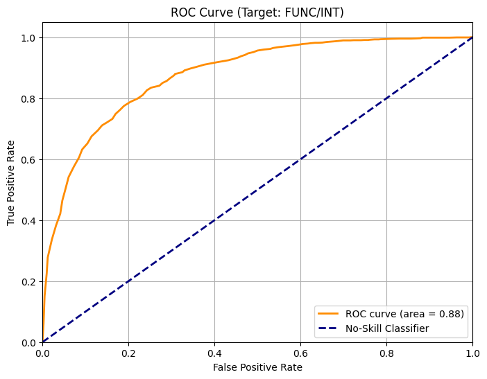
Even though we just randomly pick one layer, the improvement is significant: The AUC increases from 0.35 for the zero-shot learning to 0.88 when using embeddings.

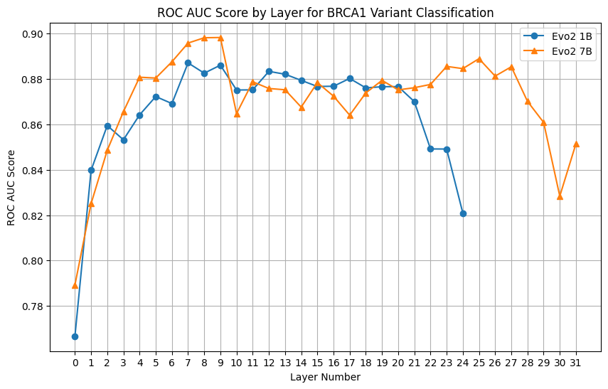
Sweeping the layers

We honestly don’t know which layer is the best, so let’s repeat the AUC calculation for all layers. Here’s the AUC values for all layers using the 1B and 7B models.

Interestingly, against the common wisdom, the best layers are among the first half of the layers. The values are quite stable as long as it is away from the first and the last layer.

Summary

To sum up, you can improve the classification performance if you can afford to learn a classifier with some data points.

Model	ROC AUC of zero-Shot learning	ROC AUC of embedding classifier
Evo 2 1B	0.73	0.89
Evo 2 7B	0.88	0.90