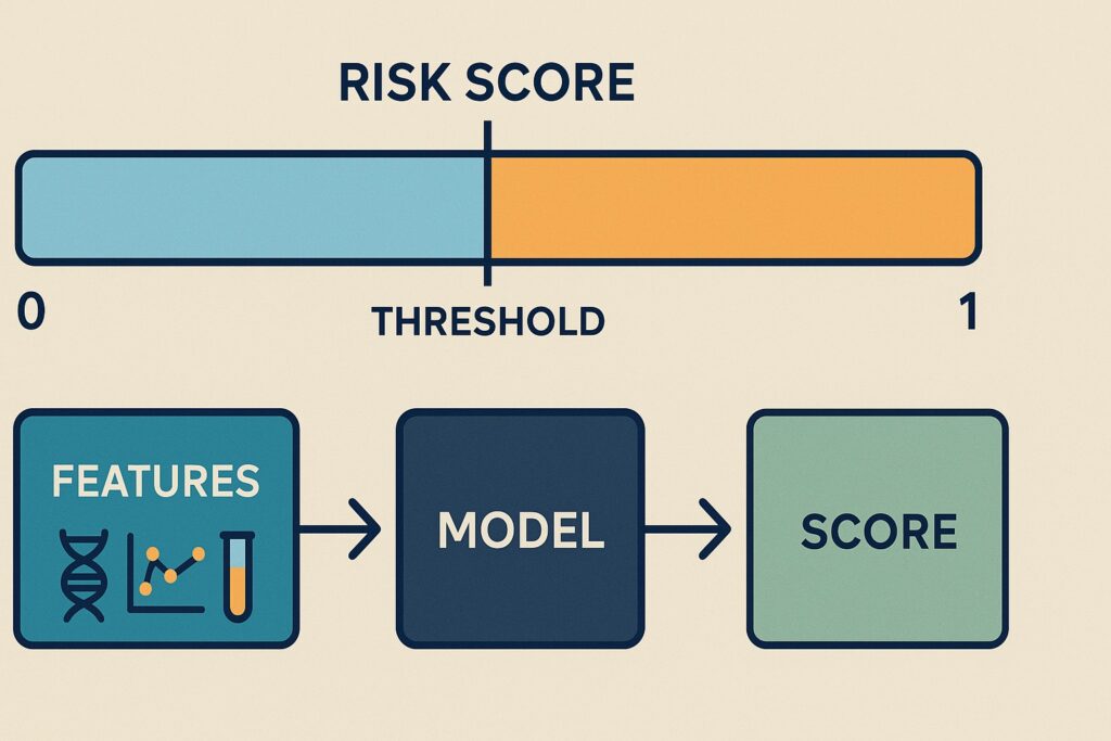
A machine learning model’s prediction for disease diagnosis is a risk score ranging from 0 to 1. We impose a decision threshold value to transform it into a Yes/No diagnosis. For example, we call cancer if the score is larger than 0.6, and non-cancer if otherwise.
How well can you trust the score? In this post, we will go through:
- The proper interpretation of the score of a machine-learning model.
- How to quantify the mis-calibration.
- Ways to calibrate the score.
Machine Learning pipeline
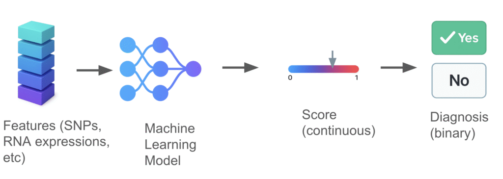
A basic machine learning pipeline consists of the following steps:
- Features extracted from the diagnostic assay are fed into the machine learning model. The features can be extracted from DNA/RNA sequencing, protein assays, or PCR. erereee eeefe
- The machine learning model processes the features and produces a predictive risk score, ranging from 0 to 1.
- A predefined cutoff, called the threshold, is applied to the score to produce a binary diagnosis. For example, if the score > threshold, the patient is predicted to have cancer. Otherwise, the patient has no cancer.
Why calibrate?
In the perfect world, a score of 0.8 means the sample has 80% chance of having cancer, and 20% chance of being normal. If you gather many samples with a score of 0.8, 80% of them are cancer and 20% of them are normal.
However, this rarely happens in practice. Instead, we need to calibrate the model, score, or threshold to achieve the expected performance.
A machine learning model makes predictions based on the training data. As part of the training process, the score cutoff is determined to give a target performance, e.g., setting the cutoff score as 0.7 for a false positive rate of no more than 1%.
Training objective
Many machine learning models learn to separate labels, but not necessarily score them properly. For example, the popular cross-entropy loss function does not guarantee proper scores.
Train-test discrepancy
A common issue with diagnostic assays is that the test data is a bit different from the training data because:
- The patient population is different, e.g., distributions of age and ethnicity.
- Batch effect: The experimental conditions, such as reagents and operators, differed slightly.
- Sample collection can vary by site or over time.
- Instrument or platform drift: The analytical measurement can change slightly over time due to the system’s condition.
- Environmental factors: The analytical measurement can be sensitive to the lab conditions, such as temperature and humidity.
Calibration can mitigate some of these factors and make the assay perform according to its specification.
Visualizing calibration
You can’t fix it if you cannot measure it. The same applies to model calibration. Measuring how much the model’s scores are off is the first step in fixing them.
You can visualize how well the scores are calibrated using a test dataset. The samples should have labels and were not used in training.
- Get the scores of the test data using the model.
- Bin the samples by the predicted scores, e.g., 0 – 0.1, 0.1 – 0.2, etc.
- For each bin, calculate the empirical score by number of positives / total number of samples.
- Plot empirical scores vs predicted scores for each bin.
Perfectly calibrated
If the scores are perfectly calibrated, you should see a plot like this:
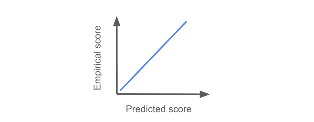
No adjustments are needed. If your scores look like this, you can close this page and do something else!
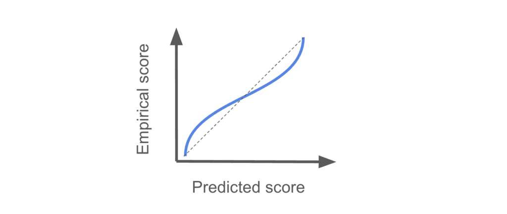
Underconfidence
We say the model is underconfident if the predicted scores are less uncertain about the label than they turn out to be.
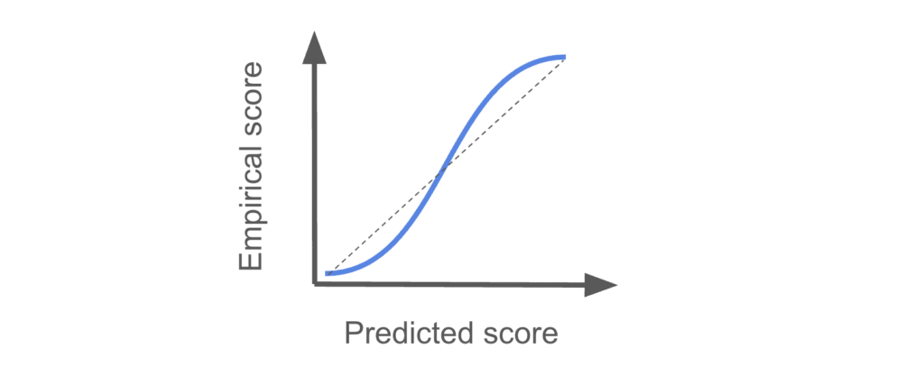
For example, a predicted score of 0.2 implies 80% chance of being a negative sample. But the empirical score is lower than 0.2, meaning that in reality it is more likely to be a negative sample than the score suggests.
Overconfidence
Similarly, the model is overconfident if it makes a prediction that is too aggressive compared to reality.
Quantifying calibration
We can use the Brier score to quantify how well the predictions match reality. For a binary classification problem like a presence/absence test, the Brier score is
\(\text{BS}=\sum_i^N (s_i – o_i)^2 \)\(s_i\) is the predicted score (ranging from 0 to 1). \(o_i\) is the observed outcome (0 or 1).
The Brier score is 0 is model makes perfect prediction. Note that it is mathematically identical to the L2 loss.
Ways to calibrate a model
Main ways to calibrate a model for binary yes/no predictions are:
- Calibrate during training: Use a loss function that encourages proper scoring during training.
- Calibrate the score: Fix the scores by learning a function map to a proper score.
- Calibrate the threshold: Learn a single scalar threshold to give desired outcome.
Calibrate during training
The idea is to train a model that produce well-calibrated scores, so that you don’t need to worry about score calibration after training.
There are several methods to achieve, or at least encourage, this during training. You can:
- Use a proper loss function such negative log likelihood.
- Add a regularization term to the objective function to encourage score calibration.
Ideally, the model is calibrated during training so we don’t need to worry about it. But this is generally difficult to achieve because your model family may not be able to represent the true distribution.
Calibrate the score
Instead, you can calibrate the score post-hoc by finding a function to map the score straight out of the model to the corrected one. The function can assume a form, such as sigmoid, or non-parametric.
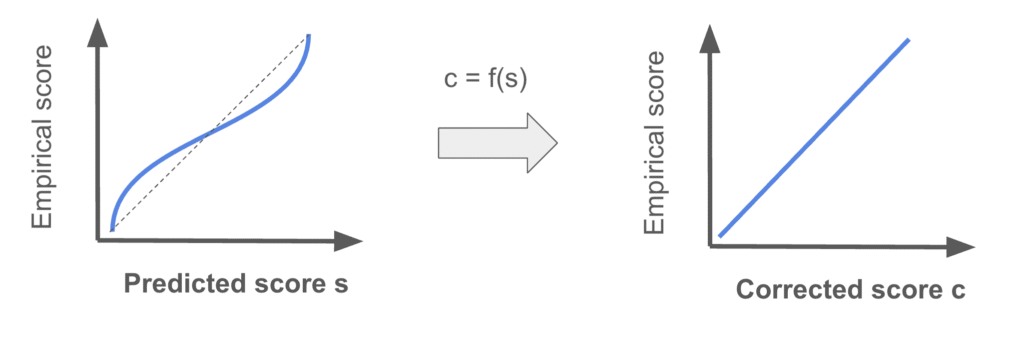
A common mapping method is isotonic regression, which fits a non-decreasing pairwise linear function.
Calibrate the threshold
If your application is simple, you can also find the scalar threshold that works for your use case directly, bypassing the score calibration. This method is called threshold calibration.
For example, you can learn the decision threshold of a cancer test using a separate calibration dataset with truth labels. This allows you to empirically determine the decision threshold to achieve 80% sensitivity, for example.